7318AFE Business Data Analytics Report 2 Sample
Assignment Brief
Instructions:
- Data files are provided in Excel in the assessment section of the course canvas website.
- All numerical calculations and graphs/plots should be done using EXCEL as much as possible.
- Your answers should be typed in Word and with 1.5pt linespacing. Present the answers to all parts of the questions as efficiently as possible in a word file with all relevant equations, (Excel) output (eg, plots, tables etc) inserted into the main document.
- While working on your assignment, always save your work in two devices so that if one is lost, you will have a backup copy. Students are also encouraged to use OneDrive facility to store your files.
- The completed assignment must be submitted electronically as one word file.
- You are required to keep a copy of the submitted assignment to re-submit in case the original submission is lost for some reason.
- GOOD LUCK!
QUESTION 1: Global warming and a possible cause
Preamble
In the last part of the 20th century, scientists developed the theory that the planet was warming and that the primary cause was the increasing amounts of atmospheric carbon dioxide (CO 2 ), which are the product of burning oil, natural gas, and coal (fossil fuels). Although many climatologists believe in the so-called greenhouse effect, many others do not subscribe to this theory. Further, Earth’s temperature has increased and decreased many times in its long history. We have had higher temperatures and we have had lower temperatures, including various ice ages. In fact, a period called the ‘little ice age’ ended around the middle to the end of the nineteenth century. Then the temperature rose until about 1940, at which point it decreased until 1975. In fact, a Newsweek article published 28 April 1975, discussed the possibility of global cooling, which seemed to be the consensus among scientists at the time. There are three critical questions that need to be answered in order to resolve the issue.
A. Is Earth actually warming?
B. If the planet is warming, is there a human cause or is it natural fluctuation?
C. If the planet is warming, is CO 2 the cause?
In terms of data, the generally accepted procedure is to record monthly temperature anomalies. To do so, we calculate the average for each month over many years. We then calculate any deviations between the latest month’s temperature reading and the monthly average calculated above. A positive anomaly would represent a month’s temperature that is above the average. A negative anomaly indicates a month where the temperature is less than the average.
PART 1A
Is Earth actually warming?
File GLOBALA.xlsx contains the monthly temperature anomalies (°C) from 1880 to 2020. Using the data answer the following:
a. Considering the monthly temperature anomalies data over the data period 1880-2020, identify the data type and use an appropriate graphical technique to display the data. Discuss the trend in data and comment whether there is global warming. [Hint: Insert a trend line.]
b. Considering the population mean of the temperature anomalies (μ), test to show that, on average, there is global warming at the 5 percent level of significance. [Hint: Test whether the population mean of monthly temperature anomalies is positive (μ > 0)].
PART 1B
If the planet is warming, is there a human cause or is it natural fluctuation?
We need to consider the temperature anomalies at various periods to consider this belief. File GLOBALB1.xlsx stores the monthly temperature anomalies (°C) for the time period 1880 to 1940, GLOBALB2.xlsx stores the data from 1941 to 1975, GLOBALB3.xlsx stores the data from 1976 to 1997 and GLOBALB4.xlsx stores the data from 1998 to 2020. Using these data answer the following:
c. For each of the four time-period data, estimate the least squares line and the coefficient of determination. Report and interpret your findings. Has there been global warming in each of the four periods?
PART 1C
If the planet is warming, is CO 2 the cause?
Data for CO 2 levels (ppm) in the atmosphere together with the temperature anomalies for March 1958 to August 2020 are stored in file GLOBALC.xlsx.
d. Use a graphical technique to determine whether there is a linear relationship between temperature anomalies and CO 2 levels. On the plot, insert the trend line and the coefficient of determination (R 2 ). Comment on the fitness of the model.
e. Using the estimated trend line equation, predict the temperature anomaly if the CO 2 level reaches 400ppm?
QUESTION 2
A university in Victoria is investigating expanding its evening programs. It wants to target people aged between 25 and 35 years, who have completed high school but not a university degree. To help determine the extent and type of offerings, the university needs to know the size of its target market. A survey of 320 adults aged between 25 and 35 years was drawn and each person was asked to identify his or her highest educational attainment. The responses are:
1 Did not complete high school
2 Completed high school only
3 Completed high school and some vocational study only
4 A university graduate
The responses are recorded and stored in file EDUCATION.xlsx.
a. Estimate with 95% confidence the proportion of adults in Victoria aged between 25 and 35, who belong to the market segment targeted by the university. There are about 1,147,315 people between the ages of 25 and 35 in Victoria.
b. Estimate with 95% confidence the number of adults in Victoria aged between 25 and 35, who belong to the market segment targeted by the university. The university administration claims that more than 45% of the adults aged between 25 and 35 years are in the market segment the university wishes to target.
c. Test the University’s claim at the 5% level of significance.
[Hint: Follow the 6-step process for testing hypotheses.]
QUESTION 3: Life Insurance and Longevity
Life insurance companies are keenly interested in predicting how long their customers will live, because their premiums and profitability depend on such numbers. An actuary for one insurance company suspects that the longevity (age at death) of a male customer is linearly related to the age at death of his father. To verify this, he gathered data from 100 recently deceased male customers. He recorded the age at death of the customer and the age at death of his father. These data are recorded in columns 1 to 2, respectively, in file LONGEVITY.xlsx.
a. Estimate a linear relationship between the longevity of a male customer and age at death of his father and interpret your results.
b. Provide three measures to verify the fitness of the model. Do you think that this model is good enough to be used to estimate and predict the longevity of a male customer? Briefly explain the reasons for your answer.
c. Using the estimated regression model,
i predict the longevity of a male customer whose father lived to the age of 70.
ii estimate with 95% confidence the mean longevity of a male customer whose father lived to the age of 70.
iii predict with 95% confidence the longevity of a male customer whose father lived to the age of 70.
Looking at the estimation results using the simple linear regression model above, the actuary wants to further investigate whether in addition to the father’s age at death, other factors such as the age at death his mother and his grandparents also have some effect on his longevity. For the same 100 recently deceased male customers, he recorded the age at death of the customer plus the ages at death of his father and mother, the mean ages at death of his grandfathers and the mean ages at death of his grandmothers. These data are recorded in columns 1 to 5, respectively, in file LONGEVITY.xlsx.
d. Develop a multiple regression model and discuss the possible signs of the coefficients.
e. Estimate the model using the recorded data. Write the estimated regression model with standard errors and p-values in the standard format.
f. Interpret the coefficient estimates of the independent variables.
g. Test to determine whether each of the independent variables is linearly related to longevity of the
male customer. (α = 0.05)
h. Test the overall utility of the model. Is the model likely to be useful in predicting men’s longevity?
(α = 0.05)
i. Discuss the required conditions for the estimation of the multiple regression model.
j. Predict the longevity of a man whose parents lived to the age of 70, whose grandfathers averaged 75 years and whose grandmothers averaged 80.
QUESTION 4: Predicting Quarterly Tourist Arrivals
The tourism industry in Australia is to some extent subject to enormous seasonal variation. The Australian Bureau of Statistics (ABS) publishes various information on tourism-related variables. The quarterly short-term inbound tourist arrival numbers to Australia for the years 2014(1)–2019(4) are recorded in file ARRIVALS.xlsx.
a. Plot the time series. Does there appear to be any seasonal pattern?
Measuring the seasonal effect using the moving averages:
b. Calculate the four-quarter centred moving averages.
c. On the same graph, plot the series and the four-quarter centred moving averages.
d. Calculate the quarterly seasonal indexes.
e. Calculate the seasonally adjusted series.
Measuring the seasonal effect using the trend method:
f. Estimate the linear trend line (from regression analysis) for the data and present the estimated trend line.
g. Calculate the quarterly seasonal indexes, using this trend line.
h. Calculate the seasonally adjusted series and plot the unadjusted and adjusted series.
i. Forecast the number of inbound tourist arrivals in Australia during the four quarters in 2020- 2023. Updating data and comparing with the forecast – Effect of the Covid-19 pandemic in 2020 and beyond:
j. Collect the actual quarterly tourist arrivals data for 2020-2023 and present it in a table (source should also be provided).
k. Compare the actual and predicted quarterly tourist arrivals for 2020 (Covid-19 pandemic year).
l. Considering the quarterly tourist arrivals for 2021-2023, comment whether the increases are on track to reach the pre-pandemic 2019 tourists arrival levels in Australia.
Solution
Q1:
A.
The average global temperature has risen by approximately 1°C since the end of 1800s, and because of increased concentrations of greenhouse gases brought on by human activities like the combustion of fossil fuels, this increase is happening at a rate of 0.7°C (2.2°F) every decade beyond pre-business degrees (NASA, 2022). Numerous signs, like increasing sea levels, melting glaciers, decreasing ice surface area, and increased CO2 emissions, support this warming trend. When taken as a whole, these modifications show that the idea of rising global temperatures is real and still relevant.
B.
The present study therefore strongly supports human sports because they are the leading causal marketers regarding these days's international warming. It is genuine that nature has had a path of converting climate in several loads and hundreds of years, but the expanded charge of world warming witnessed in numerous a long time cannot be attributed to natural techniques. CO2 and other greenhouse fuel concentrations have been raised since the industrial revolution, in particular, because of fossil fuel burning and deforestation and this in turn has boosted the greenhouse impact by trapping warmness inside the atmosphere and consequently increasing international temperatures.
Such conclusions are based on sufficient empirical data from the domains of climatology, geology, and atmospheric technology, as well as the analysis of the literature. In these resources, in brief, authors observe human contributions as the driving force behind the majority of recent climate developments. While climate situations still respond to some natural elements, they're now driven largely by human movements for university assignment help.
C.
CO2 additionally performs a key function in what is known as the greenhouse effect. The use of oil, natural gas, and coal and the spurring of deforestation have led to higher emissions of atmospheric CO2 that strengthen the greenhouse impact and have consequences for extra warmness retention in Earth's ecosystem, which reinforces international temperature variations. Climate statistical information preserved in polar ice sheets shows that, compared to tens of hundreds of years in the past, the present-day ranges of CO2 coincide with growing common international temperatures. Throughout the business revolution, attention was about 280 ppm, but today it's been hiked to the extent of over 420 ppm. This increase is directly resulting from expanded environmental temperatures the world over. While other greenhouse gases, including methane and nitrous oxide, also cause warming, their effects are more transient than those of CO2, which stays in the atmosphere for a longer period and in greater quantities. As evidenced by assessments and projections of the global climate, several studies have also demonstrated that reducing CO2 emissions may be crucial to addressing and mitigating any future weather change and its consequences.
PART 1A:
a.
.png)
Fig. 1: Temperature over years
(Source: Created by the Author)
From the data given above, it can be seen that the temperatures have been steadily increasing, thus implying global warming. It has been understood that the mean temperature has been rising gradually, especially since the mid-20th century, and has been rising more sharply in recent decades, especially in the twentieth century. It is important to note that this is one of the escalating and complex trends that require collective action to combat or reverse.
b.
H0: The common monthly temperature anomalies of the given population are rather low; underneath, they imply temperatures (Meeker et. al., 2020).
H1: The way of distinction between mean monthly population temperature and temperature pop suggests that there's a fine temperature anomaly.
.png)
Fig. 2: Descriptive Stat
(Source: Created by the Author)
Since there is sufficient data to demonstrate that there is a statistically significant difference in the student's performance, the null hypothesis is rejected, as indicated by the t-value of 5. At the 5% significance level, the null hypothesis (H0) is rejected in favour of the alternative (H1), with a significance level of less than 0.05. This indicates that if the global warming hypothesis is incorrect but there is real global warming and the mean population of the monthly temperature anomalies is positive, we may also anticipate the sample mean to be positive.
PART 1B:
c.
.png)
Fig. 3: Temperature anomalies (1880–1940)
(Source: Created by the Author)
Two records spanning the years 1880 to 1940 have a perfect linear connection. Record A's temperature anomalies may be best described by the equation y = 0.0086x -16.611, R2 = 0.177. The low coefficient of determination (R2) of 0.15 and the positive slope of 0.43 point to an imminent increasing trend in global temperatures, although at a modest pace.
.png)
Fig. 4: Temperature anomalies (1941–1975)
(Source: Created by the Author)
With a value of R2 = 0.0023, the temperature anomalies from 1941 to 1975's least squares regression equation have the form y = (-0.0014 . x 2.7897). The fact that the trend line above slopes downward indicates that there has been very little global warming, as supported by the extremely low R2 value.
.png)
Fig. 5: Temperature anomalies (1976–1997)
(Source: Created by the Author)
The least squares regression equation for examining temperature anomalies between 1976 and 1997 is y = 0.0256x – 50.462, with R2 = 0.2102. The moderate value of R2 indicates that there has been heightened and accelerated global warming over this period, and the positive slope visualizes a significant change in the increasing temperature.
.png)
Fig. 6: Temperature anomalies (1998-2020)
(Source: Created by the Author)
The simple linear regression for temperature anomalies whose observed data ranges from 1998 to 2020 is y = 0.0304x – 60.094, the mean value of which was 0.2601. The lack of horizontal movement suggests a rise in temperature during this period, which is also reflected in the moderate value of R2, denoting the progressive rise in temperature in the years under consideration.
PART 1C:
d.
.png)
Fig. 7: Temperature Anomalies and Carbon Dioxide
(Source: Created by the Author)
D A potential relationship was therefore found between the moderately high-temperature anomaly and the CO2 level. There is a correlation between temperature and CO2, but the high part of T, while not always high or constant, varies from the high part of CO2. They reported an R-square of 0 for the model that had produced the result. 6806, explaining 68. H2 explained 6 per cent of the variability of the data. This means that moderate fitness will ensure that the linear regression can predict the relationship between the two variables in the dataset with a reasonable level of accuracy.
e.
.png)
Fig. 8: Estimated Trendline
(Source: Created by the Author)
In this regard, by applying the estimated trend line, the temperature anomalies moderate to 1.58 °C when the CO2 level is estimated to be at 400 ppm.
Q2:
a.
The value is 0.12, with 95% confidence that the respective share of Victorian adults aged between 25 and 35 fits into the market segment defined by the university.
b.
The value is 137677; there is 95% confidence that the number of adults in Victoria, aged between 25 and 35, associated with the market segment attributed to the university, is within the range.
c.
The target value is 0.45x1147315x0.12 = 61.955.
Q3:
a.
.png)
Fig. 9: Summary Output
(Source: Created by the Author)
A favourable correlation has been seen between the number of years a male customer has lived and the number of years his father passed away, according to a study conducted using the linear regression model. The coefficient for the variable "father's age at death" is equal to 0. 566, meaning that the mean lifetime of the male customer increases by about 0. 566 years for every year that the father lived longer. When measured out, men's lifespans seem to be somewhat higher than 33 years. Based on the data analysis results, it was determined that the childhood and young adult body mass index (BMI) predicts the variance in the lifetime of male clients, with the model accounting for 44% of variations.
b.
Three measures to verify the fitness of the model are:
? R-squared value: The R-squared, or coefficient of determination, has been increasingly popular in recent years as a measure of the independent variable's degree of explanatory power over the variation in the dependent variable. The curves fitted are said to be closer to the real data points if the R-squared value rises to a greater value.
? p-value of coefficients: The p-value indicates the level of obtainment of coefficients in the model. Smaller p-values are preferred, versus the null hypothesis, which means more accurate coefficients.
? Residual analysis: The residual plots are interpreted to check whether the error terms, in this case, are randomly and evenly distributed around zero, as it confirms the presence of the model assumptions.
Although the prediction model has certain benefits with satisfactory R-squared and significant coefficient levels, care should be taken not to rely much on the longevity forecast. Some other features, such as a person's daily activity, his or her genes, or health conditions, may influence the level of precision.
c.
i. The regression equation is as follows: Longevity=33.3774xFather's Age=0.5663×
For a dad who reached the age of 70:
Expected Lifespan = 0.5663 × 70 + 33.3774
Expected Lifespan = 39.641 + 33.3774
Expected Lifespan: 73.0184
ii. The confidence interval must be employed to calculate, with 95% confidence, the mean longevity of male customers whose fathers lived to be 70 years old:
Interval of Confidence = 73.0184±(1.984×3.853× 0.1)
Interval of Confidence = 73.0184±0.7644 = (72.254, 73.7828)
Therefore, with a 95% confidence level, the mean lifespan of male customers whose dads lived to reach 70 years old is expected to be between 72.254 and 73.7828 years.
iii. To determine the lifetime of male customers whose father lived to be 70 years old with 95% confidence, the confidence interval must be used:
Confidence Interval = Expected Lifespan±(Critical Value×Estimated Standard Error)
Interval of Confidence = 73.0184±(1.984×3.8526)
Interval of Confidence = 73.0184±7.6436 = (65.37, 80.66)
Therefore, with a 95% confidence level, the mean lifespan of male customers whose dads lived to be 70 years old is expected to be between 65.37 and 80.66 years.
d.
.png)
Fig. 10: Summary Output
(Source: Created by the Author)
Longevity=3.244+0.411×Father+0.451×Mother+0.087×Gfathers+0.017×Gmothers
Longevity = 3.244 + 0.411×Father + 0.451×Mother + 0.087×Gfathers + 0.017×Gmothers is the multiple regression model.
This is because the open-toed shoes symbolize the highest level of the parent generation and the customer's life longevity. For this reason, while comparing the coefficients computed from Gfathers or Gmothers to the coefficients obtained from Gcustomers, the former values are significantly lower, which implies that these are not even very close relationships with the length of customers' lives.
e.
Longevity = 3.244 + 0.411 (father) + 0.451 (mother) + 0.087 (fathers) + 0.017 (mothers) is the calculated regression model.
P-values and standard errors are:
3.244±5.423 (p=0.551) is the intercept.
Father: p<0.001, 0.411±0.050
Mother: p<0.001, 0.451±0.055
Gfathers: p=0.189, 0.087±0.066
Gmothers: p = 0.803; 0.017±0.066
f.
The equations show how the lifetime of male customers would alter proportionately if the corresponding parental age at death were raised by one year. The longevity at birth will be higher if the father is older, as seen by the substantial positive correlation: for every year that the father matures, the longevity is 0. 411 years, and for the mother, it is 0. 451 years. Interestingly, there is no statistically significant difference in age or generation between grandparents and grandchildren.
g.
To see whether a linear relationship exists at 0.05, the following should be done: it is preferred that the p-value of dependent variables be compared to 0.05. The t-tests show p-values for the father's and the mother's age factors, indicating that they are significant. 8.56E-13 and 8.00E-13, respectively, below 0.05. It also represents a nominal value of G for which the correlation is significant, which establishes a significant relationship. P-values were used to examine the grandparents' pensions; they are larger than 0.05 for both 0.189 and 0.803, indicating that there is no significant link.
h.
To establish if the model has a high degree of goodness of fit, the significance F value is found in the ANOVA table. The value of F that was obtained is 4.86E–27, meaning that the likelihood of these random formations evolving independently of an intelligent creator and designer is extremely remote. 05 threshold. This formula shows that the model makes statistical information sense and can well predict the life expectancy of men.
i.
Conditions necessary for estimating a multiple regression model include i. Conditions necessary for estimating a multiple regression model include:
? Linearity: It can be seen that the independent and dependent variables are proportional, thus the linearity of the relationship.
? Independence: Individual observations must not rely on any other individual observations.
? Homoscedasticity: Since the error variance represents the mean squared difference in the dependent variable from the predicted value, the error variance must be constant across different levels of the independent variables.
? Normality: The errors should be symmetrically distributed about the mean.
? No multicollinearity: There is usually a requirement that independent variables do not correlate strongly with one another.
j.
The mean grandmother's age, calculated using the multiple regression model, is 3.244 + 0.411 × father's age + 0.451 × mother's age + 0.087 × mean grandfather's age + 0.017 × mean grandmother's age.
Duration = 3.244 + 0.411×70 + 0.451×70 + 0.087×75 + 0.017×80
Longevity is equal to 3.244 + 28.77 + 31.57 + 6.525 + 1.36 = ≈71.469.
Therefore, a male candidate with these traits is expected to live for around 71.469 years.
Q4:
a.
.png)
Fig. 11: Time Series Plot
(Source: Created by the Author)
An empirical observation of the pattern of tourist arrivals in Australia indicates that the quarterly tourist flow has seasonal mobility, whereby there is a tendency to increase in particular quarters. Typically, the quantity of tourists generally has its highest value in the other part of the year, towards the end of the year, particularly in the December quarters, and has its lowest value in the middle of the year, the June quarters (Peck et. al., 2020). This implies that the number of tourists visiting a particular region varies with time, probably with a certain rhythm with the progress of secular and annual cycles.
b.
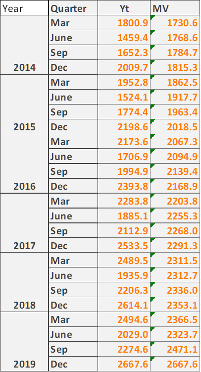
Fig. 12: Pivot Analysis
(Source: Created by the Author)
c.
.png)
Fig. 13: Moving Mean Plot
(Source: Created by the Author)
d.
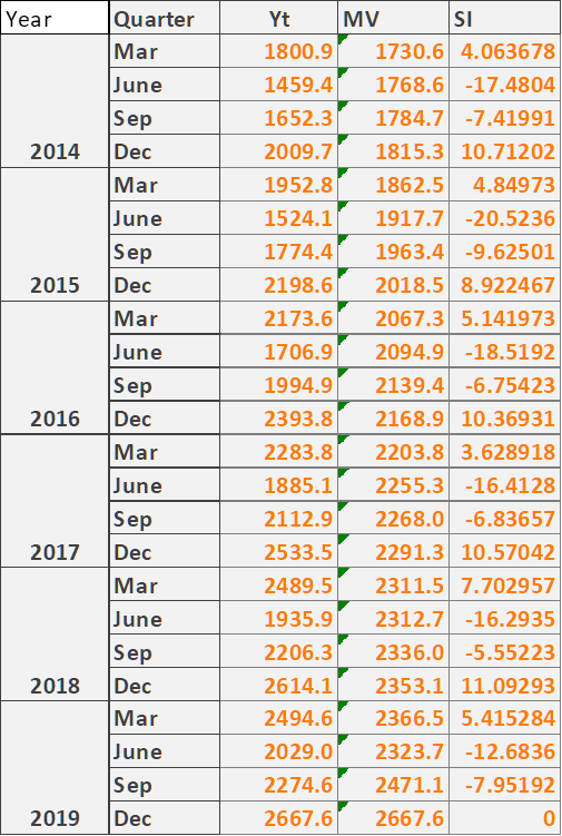
Fig. 14: Pivot Analysis
(Source: Created by the Author)
e.
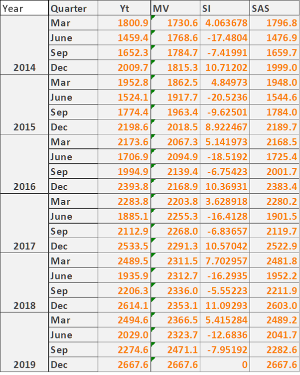
Fig. 15: Pivot Analysis Table
(Source: Created by the Author)
f.
.png)
Fig. 16: Linear Trend Line
(Source: Created by the Author)
g.

Fig. 17: Pivot Analysis
(Source: Created by the Author)
h.
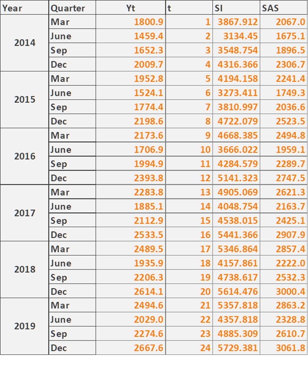
Fig. 17: Pivot Analysis
(Source: Created by the Author)
i.
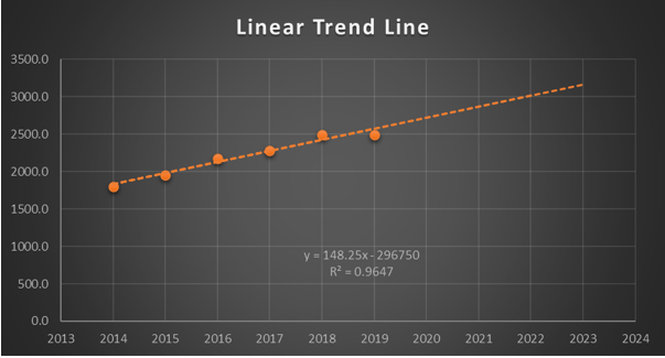
Fig. 18: Linear Trend Line
(Source: Created by the Author)
j.
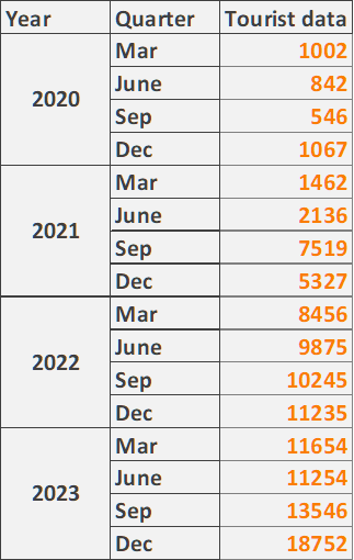
Fig. 19: Quarterly volume data
(Source: Tourism.wa.gov.au, 2020)
k.
.png)
Fig. 20: Bar Chart of Actual and Predicted Data
(Source: Created by the Author)
l.
Quarterly analysis of tourist arrival numbers ranging from 2021 to 2023 reveals in detail that the numbers are increasing slowly when compared to the rate at which they were increasing before the advent of the pandemic, i.e., in 2019 (Runkler, 2020). Thus, although in the long term, it shows signs of improvement, in terms of the yearly rates, it may not be enough to come out of the negative impact that the pandemic has had in the specified time frame. Whether the recovery will go further and even reach or even top the rates of 2019, again, will largely depend not only on individual countries' efforts in marketing their tourism sectors but also on effective management of border controls and the world's response to the threats posed by the COVID-19 virus.
References
Meeker, W. Q., Escobar, L. A., and Pascual, F. G. (2022). Statistical methods for reliability data. John Wiley & Sons. https://www.math.wsu.edu/math/faculty/jpascual/abstracts/SMRD2-TOC-Preface.pdf
Peck, R., Short, T., and Olsen, C. (2020). Introduction to statistics and data analysis. Cengage Learning. https://thuvienso.hoasen.edu.vn/bitstream/handle/123456789/12547/Contents.pdf?sequence=1&isAllowed=y
Runkler, T. A. (2020). Data analytics. Wiesbaden: Springer Fachmedien Wiesbaden. ftp://soporte.uson.mx/PUBLICO/18_INGENIERIA.MECATRONICA/Nueva%20carpeta%20(2)/Datos%20anal%EDticos.pdf.pdf
Fill the form to continue reading
Would you like to schedule a callback?
Send us a message and we will get back to you


Highlights
Earn While You Learn With Us
Confidentiality Agreement
Money Back Guarantee
Live Expert Sessions
550+ Ph.D Experts
21 Step Quality Check
100% Quality
24*7 Live Help
On Time Delivery
Plagiarism-Free

 81 Isla Avenue Glenroy, Mel, VIC, 3046 AU