HM6007 Statistics for Business Decisions/ Statistics for Managers
Assignment Brief
This assignment aims at assessing students’ understanding of different qualitative and quantitative research methodologies and techniques. Other purposes are:
1. Explain how statistical techniques can solve business problems
2. Identify and evaluate valid statistical techniques in a given scenario to solve business problems
3. Explain and justify the results of a statistical analysis in the context of critical reasoning for a business problem solving
4. Apply statistical knowledge to summarize data graphically and statistically, either manually or via a computer package Justify and interpret statistical/analytical scenarios that best fit business solution.
Group Assignment Questions
Question 1 (10 marks)
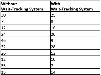
Suppose that the average waiting time for a patient at a physician’s office is just over 29 minutes. To address the issue of long patients’, wait times, some physicians’ offices are using wait-tracking systems to notify patients of expected wait times. Patients can adjust their arrival times based on this information and spend less time in waiting rooms. The following data show wait times (in minutes) for a sample of patients at offices that do not have a wait-tracking system and wait times for a sample of patients at offices with such systems. The data are stored in HI6007 Group Assignment T1 2024 data file (sheet 1).
a) Calculate the mean and median patient wait times for offices;
i. with a wait-tracking system?
ii. without a wait-tracking system?
b) Calculate the variance and standard deviation of patient wait times for offices;
i. with a wait-tracking system?
ii. without a wait-tracking system?
c) Create a box plot for patient wait times for offices;
i. with a wait-tracking system and review the information from the box plot?
ii. without a wait-tracking system and review the information from the box plot?
d) Do offices with a wait-tracking system have shorter patient wait times than offices without a wait-tracking system? Explain.
Question 2 (10 marks)
Suppose a researcher has collected sample data on beer price (in $/per litre) and per capita beer quantity consumed (in litres) in Australia between 1975-2017. The data are stored in HI6007 Group Assignment T1 2024 data file (sheet 2).
Answer the following questions
a) Prepare a numerical summary output for the two variables; beer price and per capita beer quantity consumed and explain the key numerical descriptive measures.
b) Based on the numerical descriptive measures, comment on the shape of the distribution of the two variables; beer price and per capita beer quantity consumed.
c) Test the hypothesis that the population mean per capita beer consumption is less than 135 litres/year.
d) If the researcher claims that the population mean per capita beer consumption is greater than 135 litres/year do you agree with that? Explain why.
e) Based on part (c) and (d), what can you say about the population mean per capita beer consumption in Australia?
Question 3 (20 marks)
Dixie Showtime Movie Theatres, Inc. owns and operates a chain of cinemas in several markets in the southern United States. The owners would like to estimate weekly gross revenue as a function of advertising expenditures. The data are stored in HI6007 Group Assignment T1 2024 data file (sheet 3). Using this data set and EXCEL, and no more than 1500 words in total, answer the following questions.
a) Using an appropriate numerical descriptive measure, comment on the strength and the direction of the linear relationship between weekly gross revenue and television advertising; and weekly gross revenue and newspaper advertising.
b) Develop a simple linear regression model to estimate the relationship between weekly gross revenue and television advertising expenditure and Comment on the goodness of fit of the estimated model.
c) Develop and estimate a multiple linear regression model to estimate the relationship between weekly gross revenue and television and newspaper advertising expenditure.
d) What do the estimated regression coefficients in part (c) reveal about the relationship between weekly gross revenue and television and newspaper advertising expenditure?
e) Test the overall validity of the estimated multiple regression model in part (d) at the 5% level of significance.
f) Test whether linear relationship exists between weekly gross revenue and individual independent variables in part (d) at the 5% level of significance.
g) Will your conclusion in part (f) change if the level of significance changes to 1% level of significance?
h) Compare the fitness of the multiple linear regression model with that of the simple linear regression model.
i) Based on your answers to (a) to (h) above, write a research report (of maximum 300 words) for the head of research division of your company, summarizing your findings and highlighting the managerial implications of these results?
Solution
Answer to question 1:
Part a:
i.
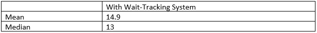
To calculate mean, excel function MEAN and for median, MEDIAN function has been used and following finding has been generated:
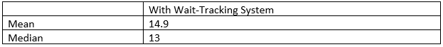
Mean patient wait time for office with wait tracking system is 14.9 and median is 13.
ii.
Mean patient wait time for office without wait tracking system is 30.4 and median is 28.
Part b:
i.
To calculate Variance, excel function VAR and for Standard deviation, STDEV function has been used and following finding has been generated for university assignment help.
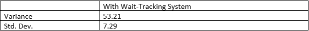
Variance of patient wait time for office without wait tracking system is 53.21 and standard deviation is 7.29.
ii.
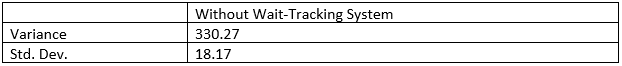
Variance of patient wait time for office with wait tracking system is 330.27 and standard deviation is 18.17.
Part c:
i.
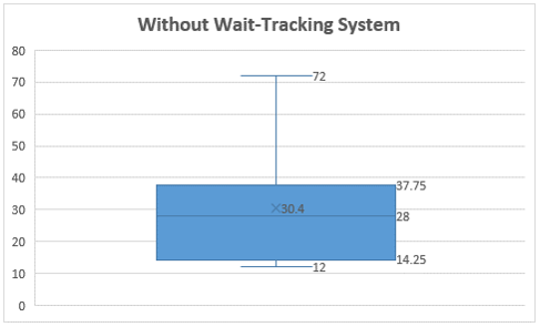
As per the box plot presented, it is observed that maximum wait time is 72 minutes, while minimum wait time is 12 minutes. Most of the offices have wait time of 28 minutes which is median, and mean is 30.4. Lower 25% of the offices has wait time of 14.24 minutes, while top 25% offices have wait time of 37.75 minutes. 50% of the offices have wait time between 14.25 minutes to 37.25 minutes where wait tracking system is not available.
ii.
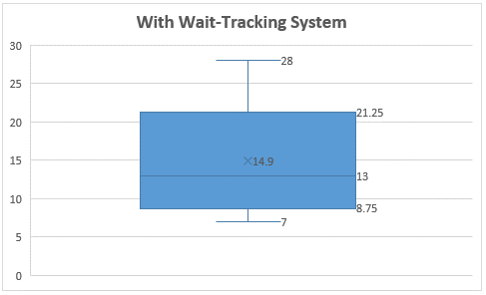
As per the box plot presented for offices with wait tracking system, it is observed that maximum wait time is 28 minutes, while minimum wait time is 7 minutes. Most of the offices have wait time of 13 minutes which is median, and mean is 14.9. Lower 25% of the offices has wait time of 8.25 minutes, while top 25% offices have wait time of 21.25 minutes. 50% of the offices have wait time between 8.75 minutes to 21.25 minutes where wait tracking system is available.
Part d:
As per the above observation mean wait time of offices with wait tracking system is lower than offices without wait tracking time. To test this, here t-test has been done at 95% confidence interval, considering following hypothesis:
• Null hypothesis (H0): Mean wait time difference is same for offices with and without wait tracking system.
• Alternative hypothesis (H1): Mean wait time for office with wait tracking system is lower than office without wait tracking system.
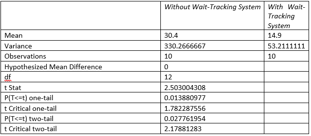
As per the t-test outcome, it is observed that p value of one tail is 0.01, which is lower than critical value of 0.05. Hence at 95% confidence level, it can be mentioned that offices with wait tracking system has lower waiting time than offices without wait tracking system.
Answer to question 2:
Part a:
To present a numerical summary of the beer price and per capita beer quantity consumed, here descriptive statistical analysis has been done.
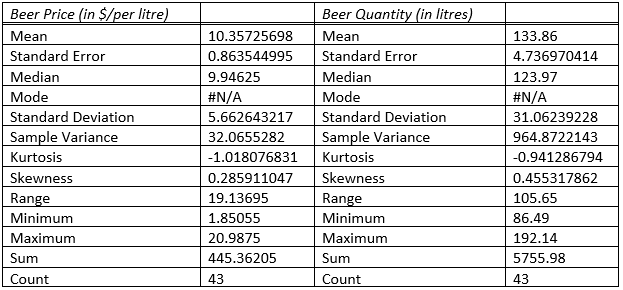
As per the Beer Price, the mean is $10.36 per litre, with a standard error of $0.86 and a standard deviation of $5.66. This showcase that the variation in the beer price is moderate. The median price is $9.95, which showcase that the prices are close to mean while with prices ranging from a minimum of $1.85 to a maximum of $20.99, a wide variation in upper and lower limit of price is observed. The price data exhibits a slight positive skewness of 0.29, suggesting a few higher values, and a kurtosis of -1.02, indicating a right tail.
As per the Beer Quantity, the mean consumption is 133.86 litres per year, with a standard error of 4.74 and a standard deviation of 31.06 litres. This showcase that the beer consumption has high variability in the data. The median consumption is 123.97 litres and difference with mean showcase, data are moderately spread from mean. With values ranging from a minimum of 86.49 litres to a maximum of 192.14 litres, wide dispersion of the data is validated. The skewness of 0.46 indicates a mild positive skew, and the kurtosis of -0.94 suggests a right tail in beer consumption data.
Part b:
As per the skewness and kurtosis value of the beer price, and beer consumption data it is observed that most beer prices are concentrated around the lower end, there are a few higher price values extending the tail to the right. Data is normally distributed for both variables.
Part c:
Null hypothesis (H0): The mean per capita beer consumption is not greater than 135 litres/year.
Alternative hypothesis (H0): The mean per capita beer consumption is greater than 135 litres/year.
Selection criteria:
• If one tail p value is greater than 0.05, null hypothesis to be accepted and alternative hypothesis to be accepted.
• If one tail p value is lower than 0.05, null hypothesis to be rejected and alternative hypothesis to be accepted.
Part d:
To test the hypothesis, here a two-sample t test considering unequal variance has been done. For doing this, a dummy variable with value of 0 has been considered.
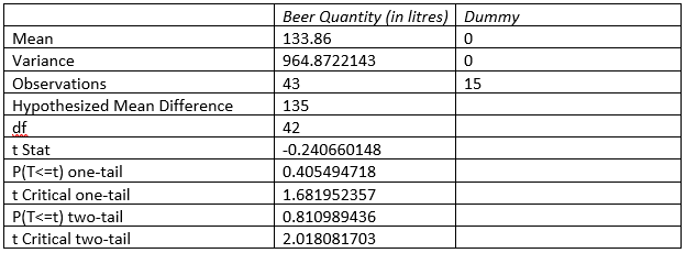
As per the t-test, it is observed that beer consumption mean is 133.86 and one tail p value is 0.40, which is much higher than critical value of .05. Hence, considering 95% confidence level, null hypothesis to be accepted and alternative is rejected. This showcase that the mean per capita beer consumption is not greater than 135 litres/year.
Part e:
As per the analysis above, beer consumption per capita in Australia is not greater than 135 litres/year. Though the beer consumption has high variability in data with wide difference between minimum and maximum value, the data is normally distributed. It has right tail, which means most of the consumers consume per capita beer close to mean, while as consumption level increase beyond mean, frequency of consumer falls.
Answer to question 3:
Part a:
To understand the strengths and directions of linear relationships between weekly gross revenue with television advertising and newspaper advertising, correlation analysis has been done. This showcases the degree of association between variables and their respective directions. Value of correlation ranges between 0 and 1, where 0 means no correlation between variables, while 1 means high correlation between variables. On the other hand, when the correlation is positive, it means a change in one variable can lead to change in other variable in same direction, while negative correlation means a change in one variable leads to opposite change in the other variable.

Following the correlation table presented above, there is a positive and high association between weekly gross revenue with television advertising and newspaper advertising. With correlation of .7533 between weekly gross revenue and television advertising, it can be inferred that a change in television advertising can lead to change in weekly gross revenue in same direction by 75.33%. On the other hand, correlation of .8931 between newspaper advertising and weekly gross revenue showcase that a change in newspaper advertising can lead to change in weekly gross revenue by 89.31% in same direction.
Part b:
To estimate the relationship between weekly gross revenue and television advertising expenditure, here regression has been done considering weekly gross revenue as the dependent variable and television advertising expenditure as the independent variable.
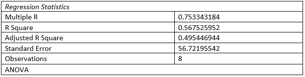
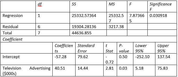
As per the regression outcome, R square value found to be .5675 which showcase that independent variable can explain 56.75% variability of the dependent variable. As per the ANOVA, F value is 7.87 and the significance level is .03. Hence the model is statistically significant at 95% confidence level and good fit to predict the weekly gross revenue.
As per the coefficient, p value for independent variable found to be 0.03, which signifies that independent variable is a valid predictor of the dependent variable. as per the coefficient, for each unit rise in television advertising expenditure, weekly gross revenue increase by $40.51. While as per the intercept term, in absence of the television advertising expenditure, weekly gross revenue would be -$57.28. Based on this, following estimation model can be formulated:
Y = -57.28 + 40.51X1 [Here, Y is weekly gross revenue and X1 is the independent variable]
Part c:
To predict the weekly gross revenue based on the television advertising and newspaper advertising, here a multiple linear regression has been done. For the regression, weekly gross revenue has been considered as the dependent variable, while television advertising and newspaper advertising has been considered as independent variable.
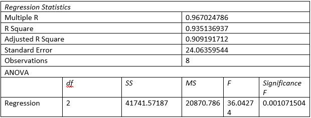
Based on the finding, following estimation model can be presented:
Y = -51.86 + 22.71X1 + 19.26X2 [here, Y is weekly gross revenue, X1 is value of television advertising expenditure and newspaper advertising expenditure]
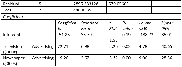
Part d:
Focusing on the coefficient table, it is observed that intercept term is -51.86, which demonstrates that in absence of the advertising expenditure, weekly gross revenue would have been -$51.86. On the other hand, both the television and newspaper advertising expenditure found to be valid predictor of the weekly gross revenue as their respective p values are .02 and .00, which is much lower than critical value of 0.05. Hence for each unit rise in the television and newspaper advertising expenditure, weekly gross revenue increases by $22.71 and $19.26 respectively.
Hence the association between weekly gross revenue and television and newspaper advertising expenditure is positive and significant at 95% confidence level.
Part e:
As per the model, R square value is .9351, which showcase that independent variables can explain 93.51% variability in the dependent variable. Moreover, F value found to be 36.04 with significance level of .00. This showcase the estimation model is good fit and independent variables can predict good amount of variability in the dependent variable.
Part f:
As per the multiple linear regression model, it is observed that a change in the independent variables can lead to significant change in the dependent variable in same direction. This showcase that as the independent variable increase, weekly gross revenue change in same direction. Moreover, the estimation model can be presented in Y = a + b1x1 + b2x2 form, where a is intercept term, b1 and b2 is coefficient term and x1, x2 are values of independent variables (Zogovi? 2023, p(63)). This association found to be good fit with high and significant F value along with high R square value.
Hence, there is a linear relationship between weekly gross revenue and individual independent variables at 95% confidence level.
Part g:
Conclusion of part f will change significantly, if the significance level becomes 1% level of significance. At 1% level of significance, critical value (p value) would become .01 (Lakens, 2022, p(16)). Hence, for independent variable whose, p value become lower than 0.01, those independent variables will then be considered as significant. Following this, as per the multiple regression outcome, p value of the television advertising is 0.02, which is higher than critical value of 0.01. Hence with 1% level of significance, television advertising then would be invalid predictor of weekly gross revenue. While as the p value of the newspaper advertising is 0.00, hence it will still be valid predictor of the weekly gross revenue.
Part h:
Comparing the fitness of multiple linear regression and simple linear regression, it is observed that single linear regression has lower R squared value (.56<.93). Moreover, adjusted R squared value is also much lower in simple linear regression compared to multiple regression. This showcase that predictability of independent variable is much higher than simple linear regression and with addition of second variable makes the model better. Standard error in the multiple regression model is much lower demonstrating better predictability of the multiple regression model compared to simple linear regression.
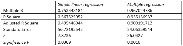
Also, as per the F value, multiple regression has higher F value with lower significance level. Though simple linear regression model also has F value higher than critical level and significance level is also lower than critical value of 0.05, high F value of multiple regression model showcase better predictability.
Hence in overall term, multiple regression model is better fit compared to simple regression model.
Part i:
The analysis aimed to assess the impact of television and newspaper advertising expenditures on weekly gross revenue. Correlation analysis revealed a positive relationship between advertising expenditures and revenue, with television advertising showing a correlation of 0.7533 and newspaper advertising a higher correlation of 0.8931, indicating stronger revenue influence. Simple linear regression indicated that television advertising alone explains 56.75% of the revenue variability (R² = 0.5675), with each $1,000 increase in spending leading to a $40.51 revenue increase (p = 0.03). Multiple linear regression, which included both advertising types, significantly improved model fit (R² = 0.9351), demonstrating that combined advertising expenditures explain 93.51% of the revenue variability. The coefficients for television and newspaper advertising were $22.71 (p = 0.02) and $19.26 (p < 0.001) respectively, for each $1,000 spent.
These findings have several managerial implications. First, the high R² and significant results underscore the importance of allocating budgets to both television and newspaper advertising to drive revenue. Notably, newspaper advertising, with its higher correlation and coefficient, should be a focal point for increasing revenue. The regression models provide a robust framework for predicting revenue changes based on advertising expenditures, aiding strategic planning and budget allocation. Furthermore, while both advertising mediums are significant predictors at a 5% confidence level, only newspaper advertising remains significant at a 1% level, suggesting a more reliable impact on revenue.
Reference:
D Lakens 2022, ‘Sample size justification’, Collabra: psychology, 8(1), p.33267. https://research.tue.nl/files/214011492/collabra_2022_8_1_33267.pdf
K Zogovi? 2023, ‘Revealing hidden trends: investigating product sales patterns with categorical and continuous predictors in a distinctive dataset’. Science International Journal, 2(3), pp.61-67. https://scienceij.com/index.php/sij/article/download/26/33
Fill the form to continue reading
Would you like to schedule a callback?
Send us a message and we will get back to you


Highlights
Earn While You Learn With Us
Confidentiality Agreement
Money Back Guarantee
Live Expert Sessions
550+ Ph.D Experts
21 Step Quality Check
100% Quality
24*7 Live Help
On Time Delivery
Plagiarism-Free

 81 Isla Avenue Glenroy, Mel, VIC, 3046 AU